By Joseph Profeta Ph.D., Director – Control Systems Group, Aerotech
 As servo systems contain error-driven control loops, tuning is an integral component of any successfully commissioned machine or plant, especially because it has a direct impact on performance. A correctly tuned servo system can enhance important process parameters such as stability, precision and productivity, but how is it best to achieve these outcomes?
If inherent system resonance becomes excited during a process or operation, instability will likely ensue. In most cases, if the motor safety parameters are set up correctly, this issue will result in little more than an audible noise and an error message indicating that the motor has received too much current, thus disabling the axis. However, in some cases, it can lead to mechanical damage which occurs when uncontrolled motion slams the load into the hardstop causing process disruption. The cost of poor tuning can be seen in significantly slower production rates and possible equipment damage.
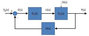
Before thinking about potential tuning solutions, a review of the general problem will prove beneficial. Consider an application example which requires the control of the output of an inertial mass so that a machine can perform a movement in a specific direction, or to a set position (where a sensor measures the output feedback). Subtracting the feedback signal (Y) from the desired signal (Yd), results in an error signal (E), which the controller can act upon to provide the machine with an actuation signal (U). If the controller is stable and robust, the output will track the desired input in the presence of both external disturbances (D) and some plant variation. Typical system outputs controlled are position, velocity, current, or force but any system variable that can be measured (or at least estimated) can be subjected to closed loop control. Often, the tuning process takes place in the time domain, but engineers can benefit by using the frequency domain to further improve performance.
A common question is why the need exists for a closed loop system. Put simply, the presence of system errors, which emanate from sources such as friction, mass imbalance, sensor error, electrical noise, cogging/ripple torque, plant variation and environmental disturbances will affect the system output in undesirable ways. If these error sources did not exist, open loop control would work well.
Time or frequency domain?
Most are familiar with standard PID controllers, and aware of how the system step response output will change as the different gains are increased or decreased. Although this is a fairly common operation, the problem with the time domain is a general absence of any real understanding about the character of the resonance structure that needs controlling.
Using the frequency domain for tuning provides more information, which, when used in conjunction with the time domain information, can result in optimal servo system performance for the specific motion required of the system.
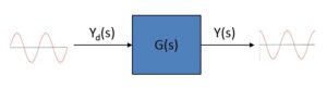
In basic terms, a frequency response is the steady-state response of a system to a sinusoidal input. For linear systems, the output will have the same frequency as the input frequency, but may have a different magnitude and phase. At each frequency, the output magnitude and phase is compared to the input magnitude and phase. The magnitude and phase of this comparison is plotted against frequency – which is called a Bode plot. Most controllers have tools for measuring the frequency response of a system. There are several methods for collecting the frequency response with the most common being discrete sinusoids, white noise and multi-sine methods.
Bode plots are not the only frequency domain tool used in control systems. Often FFTs (Fast Fourier Transforms) are used to study frequency content in a time signal. This can be useful in finding the frequency of an oscillation. The Bode plot will provide more information such as the width and depth of the resonance and most importantly the resonance effect on the stability of the system.
Applying the tools
To apply the tools it is useful to have a model of the system. By thinking of the system as a set of masses connected by springs and dampers, it is possible to create a mathematical model of the system which can be used to predict the response of the system to a specific input, such as a step. The model complexity increases with the number of masses considered. For this reason, often a two-mass model is sufficient to predict first order responses and can be used for insight into how to tune the system.
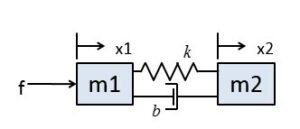
Consider a linear axis with a load that needs to be positioned accurately. The task at hand is to control the position of the second mass based on the force applied to the first mass. The position of Mass 2 will depend on the effects of the spring, damper, relative ratio of the masses and any disturbances in the system, such as the friction created by bearings or errors due to the sensor measuring the position of Mass 1. It is not always possible or cost-effective to measure the position of Mass 2.
When considering the reaction of the system to an input, there are two frequency domain parameters of interest: bandwidth and damping. A higher bandwidth is synonymous with a faster rise time and better overall system performance, while decreasing damping equates to more oscillation. High bandwidth and low damping usually imply higher machine throughput.
Loop gain: pathway to stability
When enabling an axis, uncontrollable slamming into the hardstop usually leads us to consider tuning the system. However, the presence of high pitch in a system may also indicate an instability. Of course, it is preferable to tune the system such that it is robust, eliminating high pitches, oscillations and uncontrolled movements. When using the time domain, this is not always possible without unnecessarily lowering the performance of the system by reducing bandwidth of a low pass filter until the resonant response is sufficiently dampened. By using the frequency domain it is possible to optimise notch filters to dampen the resonant response and keep the bandwidth higher than when just using the time domain tuning techniques.

To do this, the loop transmission response (or loop gain) is used. Theoretically, as long as there is a small amount of gain and phase margin, the system will be stable. Practical values for a robust system are a gain margin of at least 6 dB and a phase margin of at least 30°. The Gain margin is the difference from the 0 dB line to the gain curve at the frequency where the phase crosses 180°. The Phase margin is measured from the phase curve to the 180° at the frequency where the loop gain crosses the 0 dB line.
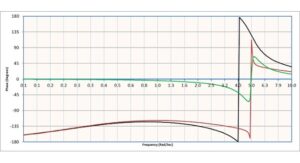
In a practical example of using the frequency response domain, consider the loop transmission of a system exhibiting a resonance at 5 rad/sec. Here, technicians can use a notch filter of similar depth and width to cancel out machine resonance. Note, the resonance still exists in the mechanical system, meaning the potential exists to excite it, but the instability will be dampened by the notch filters and not destabilise the system.
With the ‘notching out’ of resonance from the control loop, it becomes possible to increase overall system gain, extend bandwidth to provide faster rise times and, ultimately, increase machine performance. Below the plant is red, the notch filter is green, and the resulting response is black.

Whenever performing stabilisation, a good objective is to aim for maximum bandwidth and minimum phase loss as it nearly always provides the optimum outcome, although in practice, some level of judgement is usually required to determine the acceptable margin. When looking at a loop transmission plot, it is important to not only examine the phase crossover frequencies for sufficient gain margin, but areas around those points for low gain margins.
Loop shaping, step by step
Before starting to tune, do not forget to tighten all the bolts and level the machine. The following steps generally apply when tuning an inertial mass.

For the control loop structure shown above, the initial tuning step is setting the gains Kpos and Kp to very low values with Kp = 10 Kpos and Ki = 0. Then use the standard autotune tool set to a low bandwidth to get a good starting point for loop shaping. Autotune will stimulate the system with a series of sinusoids and calculate a basic set of gains with sufficient stability to run a loop transmission.
After collecting a loop transmission, identify the point of maximum phase in the plot, then maximize the crossover frequency based on the slope of the phase plot by increasing the magnitude response. Here, be wary of resonant modes at low-to-mid frequency and keep an eye on the gain margin.
The next task is to introduce a low-pass filter. Set the frequency of the filter as high as possible to lose as little phase margin as possible, but low enough to suppress sensor noise. However, take care to ensure the filter is not set too low as it will reduce machine performance. A good rule of thumb is to apply a low-pass filter at approximately 10 times the crossover frequency, which will avoid phase loss.
Next, apply a notch filter on the centre frequency of any resonance. Adjust the depth and width of the notch to sufficiently flatten the gain curve at the notch. It should now be possible to raise the gain curve while maintaining sufficient gain margin and phase margin. Positive outcomes will include greater bandwidth, better stability of the axis, and higher machine throughput since it will have a faster response time to input signals.
For best practice, use the time domain again to see how the system responds to specific machine operations, such as contouring. Repeat this step as necessary. Also this process should be repeated at different operating points of the system including a variety of locations and current levels.
Loop shaping on the system has many benefits, not least the use of measured data rather than analytic models to understand the resonant character of the system, the provision of insight into non-linear effect, quantitative stability measures and, most importantly, improved system performance over tuning in the time domain alone.

For further information visit www.aerotech.com.
Aerotech – Dedicated to the Science of Motion
Aerotech Inc., based in Pittsburgh, USA, is a privately held, family-owned company founded in 1970 by Stephen J. Botos with the vision of advancing the science of motion control and positioning systems for customers in industry, science and research. As a family business, the owners continue to place great value on open and trusting relationships with customers, business partners and employees. In Germany, the mid-sized company is represented by its own subsidiary, Aerotech GmbH, based in Fürth. In addition to sales and service activities, the Fürth facility handles customised assembly of positioning systems for the European market. The company’s innovative and high-precision motion solutions meet all critical requirements necessary for today’s demanding applications. They are used wherever high throughput is required – including medical and life science applications, semiconductor and flat screen production, photonics, automotive, data storage, laser processing, aerospace and electronics manufacturing, as well as inspection, testing and assembly.
With advanced analysis and diagnostic capabilities, Aerotech provides world-class technical support and service. If a standard product is not suitable for an individual application, Aerotech can supply special motion components and systems based on its many years of expertise and experience. Manufacturing capacity for customer-specific applications is supplemented by experience in supplying systems for vacuum and clean room operation.
Aerotech has full-service subsidiaries in Germany (Fürth), United Kingdom (Ramsdell), China (Shanghai) and Taiwan (Taipei). Aerotech currently employs around 500 people worldwide http://www.aerotech.co.uk